Open Problem: Learning sparse linear concepts by priming the features

Manfred K. Warmuth and Ehsan Amid MANFRED,EAMID@GOOGLE.COM, Google Inc.

Editors: Gergely Neu and Lorenzo Rosasco

Abstract

Sparse linear problems can be learned well with online multiplicative updates. The question is whether there are closed-form updates based on the past examples that can sample efficiently learn such sparse linear problems as well?

We show experimentally that this can be achieved by applying linear least squares, then "priming" the $i$th features of the past instances by multiplying them by the $i$th linear least squares weight, and finally applying linear least squares a second time. However, it is an open problem whether such priming methods have provably good regret bounds when applied online.

Keywords: multiplicative updates, gradient descent, relative entropy regularization, linear least squares, ridge regression, rotation invariance, kernel methods, regret bounds.

1. Introduction

Sparse linear problems can be learned with online multiplicative updates. It all started with Winnow (Littlestone, 1988), which learns $k$ out of $n$ disjunctions with a regret bound of $O(k\log n)$ mistakes. Later this was generalized to sparse linear regression (Kivinen and Warmuth, 1997) using the Exponentiated Gradient update for the square loss. Now sparsity is roughly characterized by the number of non-zero weights in the target weight vector. Essentially the regret bounds still grows logarithmically with the input dimension $n$. More precisely, the square loss regret for noise-free linear regression is $O(W_1^2 X_\infty^2 \log n)$ where $W_1, X_\infty$ are bounds on the 1-norm of the target weight vector and the infinity norm of the instances, respectively. The Exponentiated Gradient (EG) update (Winnow is a special case when the loss is the hinge loss) is motivated by relative entropy regularization (Kivinen and Warmuth, 1997). In contrast, the gradient descent (GD) family of updates, including Ridge Regression, are based on the Euclidean distance squared regularization. The resulting updates are rotation invariant (Warmuth and Vishwanathan, 2005; Warmuth et al., 2014) in that rotating the instances and initialization leave the updates and predictions unchanged. This rotation invariance has the side effect that the gradient descent family for single linear neurons is suboptimal for learning sparse problems. When the instances are dense, then the regret bounds are linear in $n$.

Kernelization of the GD type update does not help (Warmuth and Vishwanathan, 2005) and recently it was also shown that underconstrained sparse linear problems cannot even be efficiently learned with any GD trained neural net that has a fully-connected bottom layer and is rotation invariantly initialized. The key is again that GD updates on such networks are rotation invariant.

The difference between the two regularizations seemed insurmountable. But recently it has been shown that multiplicative updates can be reparameterized approximately¹ as GD updates on a "spindly" two-layer network (Amid and Warmuth, 2020a; Chizat, 2022) (Each edge in the linear neuron is replaced by a double edge). These updates access individual features (as multiplicative updates do) and are decidedly not rotation invariant.

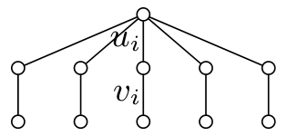Figure extracted from page 1 of the published PDF (300 DPI crop).

Essentially the same regret bounds have been proven for sparse linear regression with the GD update on the spindly network and for the GD approximation of Winnow on the same network for learning disjunctions (Amid and Warmuth, 2020b), thus solving the COLT open problem of Warmuth (2006).

The big advantage of the GD family is that it has closed-form solutions for second-order updates such as for Linear Least Squares (LLS) and Ridge Regression (RR). Regret bounds have also been proven for LLS (Vovk, 1997; Forster, 1999; Azoury and Warmuth, 2001) which are linear in the feature dimension $n$. No closed-form updates exist for relative entropy regularization whose regret grow with $\log n$. Here we propose such closed-form updates by essentially applying LLS twice.

Besides the large body of work in online learning, there are other lines of research on sparse target recovery from a small sample (e.g., Needell and Tropp (2008); Yasuda et al. (2023)). The open problems of this note focus on simple one-stage priming and evaluating the updates with worst-case regret bounds.

2. Priming for the underconstrained noise-free sparse linear regression

The multiplicative updates (& approximations) for a single example $(\boldsymbol{x}, y)$ with square loss are:

For all but Approximated EGU, there are regret bounds of $O(k\log\frac{n}{k})$ when the target is the average of $k$ out of $n$ features and the features have bounded range.

Priming setup: The past linear regression examples $\{(\boldsymbol{x}_i, y_i)\}$ are denoted in matrix notation as $(\boldsymbol{X},\boldsymbol{y})$, where $X(i,:) = \boldsymbol{x}_i^\top$.

In feature priming, the $i$th feature is multiplied by the prime factor $p_i$ and then LLS is applied:

The question is, what are good priming² factors $p_i$? The goal is to obtain methods that are close to optimal for both sparse & dense linear problems. Note that to learn sparse linear, priming must break rotation invariance by emphasizing "good" features. The online updates and the below three priming methods do this in different ways:

1. $p_i = \operatorname{argmin}_{p_i} (\boldsymbol{X}(:,i)\,p_i - \boldsymbol{y})^2 = X(:,i)^\dagger\boldsymbol{y} = \frac{X(:,i)^\top}{\|X(:,i\|^2}\,\boldsymbol{y}$ (1-dim LLS per $i$th feature)

2. $p_i = \frac{(X(:,i)-\overline{X(:,i)})\,(\boldsymbol{y}-\overline{\boldsymbol{y}})}{\sqrt{(X(:,i)-\overline{X(:,i)}}\sqrt{\boldsymbol{y}-\overline{\boldsymbol{y}}}}$ (Pearson correlation coefficients)

3. $\boldsymbol{p} = \boldsymbol{w}_{\mathrm{LLS}} = \boldsymbol{X}^\dagger\boldsymbol{y} = (\boldsymbol{X}^\top\boldsymbol{X})^\dagger\boldsymbol{X}^\top\boldsymbol{y}$ (Simplest method: LLS for priming as well)

See Figure 1 for an experimental comparison. If priming is powered up with primepower$= 2$ (i.e. $\boldsymbol{p} = \operatorname{sign}(\boldsymbol{p}) \mathbin{.*} |\boldsymbol{p}|.^{\text{primepower}}$), then these methods converge even faster on sparse targets (Not shown).

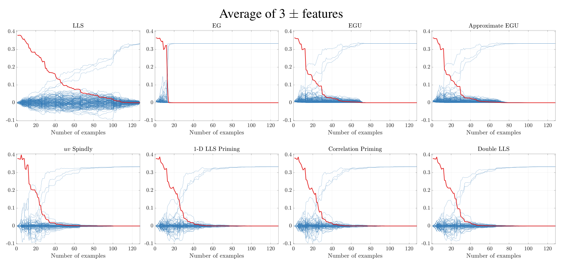Figure extracted from page 3 of the published PDF (300 DPI crop).

Figure 1: We draw a random $n \times n$ $\pm1$ matrix $\boldsymbol{X}$, with $n = 128$. The rows are the $n$ instances and the sparse label vector $\boldsymbol{y}$ is the average of the first three column features. After seeing $t = 1 : 128$ examples, we plot weights (in blue) after applying LLS or the priming methods to all examples. For the online update, we do multiple passes over the past examples until the weight vector is consistent (EGU$\pm$ is a 2-sided version of EGU). In red, we always plot the average square loss on all 128 examples. LLS picks up the target weights too slowly. Multiplicative updates do this much faster. All three priming methods perform similarly to the multiplicative updates. When the target vector $\boldsymbol{y}$ is the average over 3/4 of the features (i.e., dense), then the loss curve of all methods is similar to the loss curve of LLS (Not shown).

Open Problem 1 Are there competitive regret bound for any of the priming methods?

Open Problem 2 What is the optimal priming function for sparse linear problems?

Open Problem 3 Are there priming methods for learning sparse disjunctions?

3. Priming for the overconstraint case

Let's focus on our simplest priming method based on doing LLS twice. In the noisy case, we will prime with LLS but the "outside" weight computation must be done with $\lambda$ Ridge Regression. When $\lambda$ is tuned you hit the bottom of the loss curve dip of the multiplicative updates (Figure 2). We conclude with a final open problem about priming. LLS and Ridge Regression can be kernelized, i.e., kernels efficiently but implicitly operate in a typically much larger feature space. Is it possible to approximately prime in feature space and then do the weight computation using the primed kernel?

Open Problem 4 Can kernels be primed efficiently?

4. Upping the ante: The single example problem.

Assume you have $\pm 1$ instances and the target label is the first feature. Now "stretch" the first feature and label by multiplying both by a factor of 1.2. This has the effect that EG, when trained to consistency, makes use of the fact that the target is normalized and homes into the unit target vector $\boldsymbol{e}_1$ after seeing a single example. However, we have no priming-based method that can achieve this.

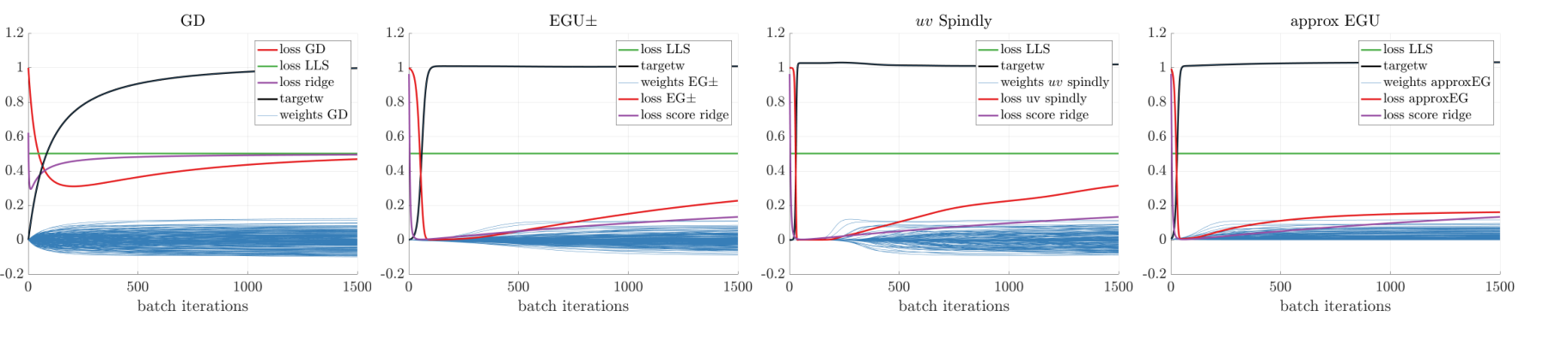Figure extracted from page 4 of the published PDF (300 DPI crop).

Figure 2: Now the number of examples is a 10 fold multiple of the feature dimension $n = 128$ and the target is a single feature plus random noise. The x-axis is the number of passes over the entire batch of examples. All methods benefit from early stopping (i.e., the red excess loss curves over the loss of the target feature all have a dip). Tuned Ridge Regression (overlayed in purple) hits the bottom of the dip of the GD loss curve. Similarly, tuned Ridge Regression, when primed with LLS, hits the much lower dip of the multiplicative updates.

5. Conclusion

Back to online updates. Multiplicative updates are also used for obtaining $O(\log n)$ regret bound for the expert setting w.r.t. a large variety of losses (Vovk, 1990; Haussler et al., 1998). The Randomized Weighted Majority / Hedge update and bounds have already been "spindlified" (Amid and Warmuth, 2020b). For the expected log loss (i.e. when the expert algorithm is Bayes rule), this is not possible.

Open Problem 5 For which other other losses can the expert algorithm be spindlified?

We have regret bounds already for some of the online updates such as EGU and its spindlified version. But note that all these updates do some sort of priming: EG exponentiates the gradients. Spindly and Approximated EGU multiply the gradient by the current weight vector. For example, the simplified $\boldsymbol{u}\odot\boldsymbol{u}$ spindly minimizes $(\boldsymbol{X}\boldsymbol{u}\odot\boldsymbol{u}-\boldsymbol{y})^2$ with GD and its batch gradient is:

Setting the gradient to $\boldsymbol{0}$ has many solutions: $\boldsymbol{u} = \sqrt{\operatorname{diag}(\boldsymbol{p})^\top(\boldsymbol{X}\operatorname{diag}(\boldsymbol{p}))^\dagger \boldsymbol{y}}$. Spindly is motivated by Euclidean square regularization. So in the noise-free case, it is natural to consider the following limit:

Open Problem 6 What does spindly converge to? Does it have a closed-form solution?

Why is this question important? Euclidean squared regularization has a closed-form batch solution as Ridge Regression. However, the GD family of updates cannot learn sparse targets well. Multiplicative updates (motivated by relative entropy regularization) handle sparse targets very well but have no closed-form batch solutions due to the exponentiation of the gradients. However an approximated closed-form minimum relative entropy solution with good regret bounds might be obtainable via the spindlification method and the new priming methods introduced here.

Finally, one-norm regularization is a common way to retrieve sparse solutions (Yasuda et al., 2023) and in Hoff (2017) a version of $\boldsymbol{u}\odot\boldsymbol{v}$ spindly is motivated this way. If the spindly updates have an alternated one-norm motivation, then the following picture emerges: multiplicative updates are approximated by the spindly one-norm updates and the priming methods introduced here are a further two-stage closed form approximation. The overall question is, what is the commonality of all these learning methods for sparse targets and which one is the most effective and practical for learning with neural networks?

Acknowledgments

Thanks to Jake Abernethy, Alekh Agarwal, Matt Jones, Wojciech Kotłowski, Teodore Marinov, and Taisuke Yasuda for many inspiring discussions.

References

Ehsan Amid and Manfred K. Warmuth. Reparameterizing mirror descent as gradient descent. In Proceedings of Advances in Neural Information Processing Systems, volume 33, pages 8430–8439, 2020a.

Ehsan Amid and Manfred K. Warmuth. Winnowing with gradient descent. In 33rd International Conference on Algorithmic Learning Theory (COLT), pages 125:163–182. PMLR, 2020b.

Katy Azoury and Manfred K. Warmuth. Relative loss bounds for on-line density estimation with the exponential family of distributions. Journal of Machine Learning, 43(3):211–246, June 2001.

Lénaïc Chizat. Convergence Rates of Gradient Methods for Convex Optimization in the Space of Measures. Open Journal of Mathematical Optimization, 3:8, 2022. doi: 10.5802/ojmo.20.

Jürgen Forster. On relative loss bounds in generalized linear regression. In 12th International Symposium on Fundamentals of Computation Theory (FCT '99), pages 269–280. Springer, 1999.

David Haussler, Jyrki Kivinen, and Manfred K Warmuth. Sequential prediction of individual sequences under general loss functions. IEEE Transactions on Information Theory, 44(5):1906–1925, 1998.

Peter D. Hoff. Lasso, fractional norm and structured sparse estimation using a hadamard product parametrization. Computational Statistics & Data Analysis, 115:186–198, 2017.

Jyrki Kivinen and Manfred K. Warmuth. Exponentiated gradient versus gradient descent for linear predictors. Information and Computation, 132(1):1–63, 1997.

Nick Littlestone. Learning quickly when irrelevant attributes abound: A new linear-threshold algorithm. Machine learning, 2(4):285–318, 1988.

Deanne Needell and Joel A. Tropp. Cosamp: Iterative signal recovery from incomplete and inaccurate samples, 2008. ArXiv:0803.2392.

Volodimir G Vovk. Aggregating strategies. In Proceedings of the third annual workshop on Computational learning theory, pages 371–386, 1990.

Volodya Vovk. Competitive on-line linear regression. In Advances in Neural Information Processing Systems, volume 10. MIT Press, 1997.

Manfred K. Warmuth. Can entropic regularization be replaced by squared euclidean distance plus additional linear constraints. In 19th Annual Conference on Learning Theory, pages 653–654. Springer Verlag, June 2006.

Manfred K. Warmuth and S.V.N. Vishwanathan. Leaving the span. In Proceedings of the 18th Annual Conference on Learning Theory (COLT), pages 366–381, 2005.

Manfred K. Warmuth, Wojciech Kotłowski, and Shuisheng Zhou. Kernelization of matrix updates. Journal of Theoretical Computer Science, 558:159–178, 2014.

Taisuke Yasuda, Mohammadhossein Bateni, Lin Chen, Matthew Fahrbach, Gang Fu, and Vahab Mirrokni. Sequential attention for feature selection. In The Eleventh International Conference on Learning Representations, 2023.